How to Know a Scrub Jay is a Scrub Jay
Elias Castro
March 29, 2024
Have you ever wondered how to train a computer to listen to a certain sound amongst others? How could you classify it? How could you do it on an embedded system that has limited space and power? These were all the questions we had to ask ourselves when figuring out how to identify a Scrub Jay.
To give more context, when a tag is attached to a Scrub Jay there is a microphone on it. The purpose of this microphone is to listen to the calls that a Scrub Jay makes. In a perfect world, this call would have no outside noise and one could easily identify it. In reality, there will be noise at every possible moment, from the sounds of the wind and the rain to the sounds of other birds and the Scrub Jay itself rustling through trees. So now comes the big question: if you were a computer, how could you tell when a Scrub Jay is present?
For starters, a computer sadly can't hear, so it must rely on another piece of information: PCM data. PCM stands for Pulse Code Modulation, which is a method used to digitally represent analog signals such as audio. The signal is continuously sampled at regular intervals where the amplitude is then encoded as binary numbers. These values can then be stored in an array where each index represents one sample and each value represents the signal's amplitude. Let's take a look at one audio sample where the Scrub Jay is making a call and visualize it:
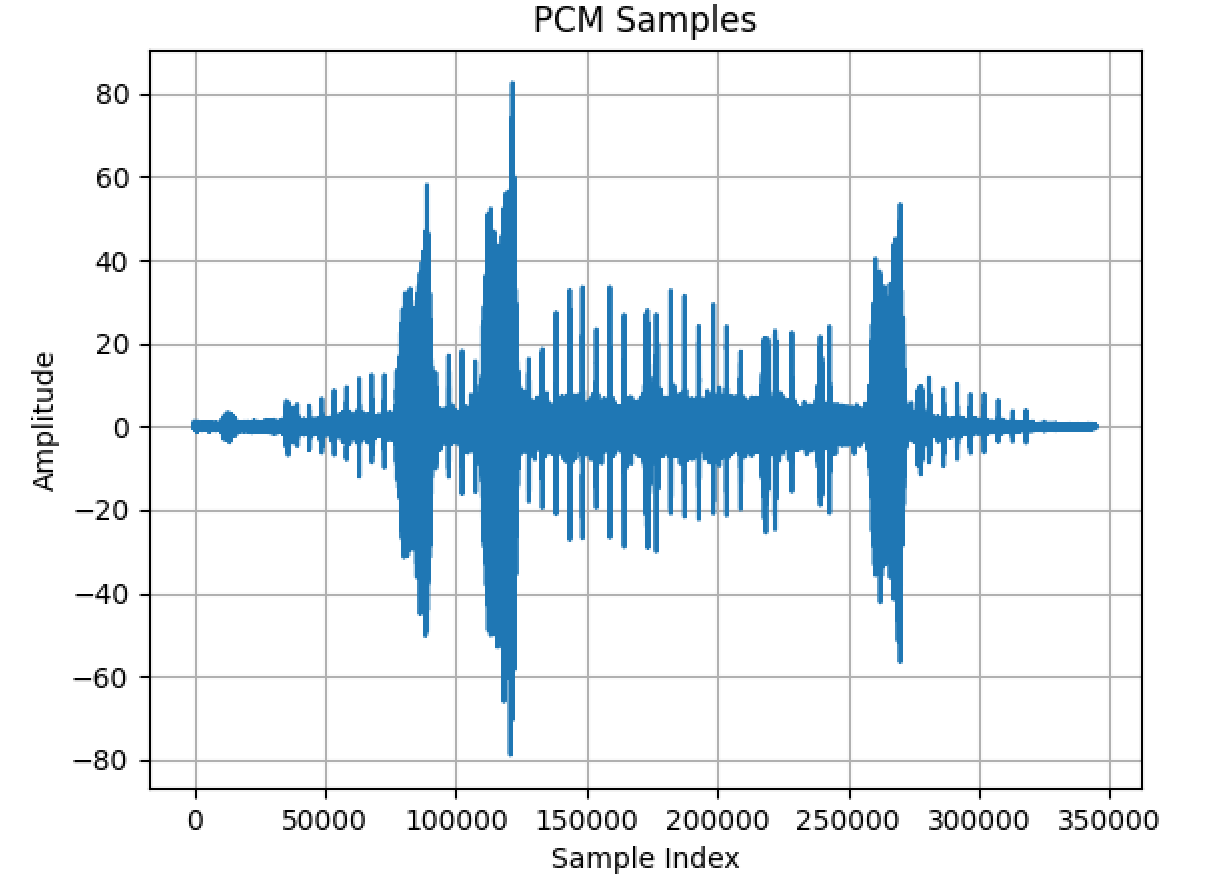
PCM samples of a Scrub Jay with noise
In this audio, the Scrub Jay is clicking, which explains the constant increase and decrease of the amplitude throughout the figure. Next, notice the three large spikes that are out of place. This is the sound of another bird calling in the background, which we would classify as noise since this is not the sound we are looking for. To compare, let's take a look at another audio sample that has little to no noise. In this audio, the Scrub Jay is making the same clicking noise:
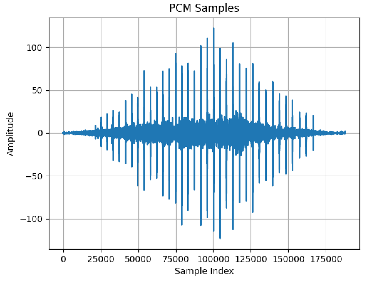
PCM samples of a Scrub Jay with no noise
Notice how the pattern is strikingly similar to Figure 1! The amplitude constantly increases and decreases throughout the indexes. This is the pattern that we want to look for when we have noisy audio such as the previous one.
Great, we know the audio pattern that we have to look for! Now we tackle the next question: how can we classify a Scrub Jay with our tag? Remember that our tag is an embedded system, meaning that there are physical, power, and memory constraints that we must adhere to. Unfortunately, we cannot use something as powerful as a support vector machine (SVM) to train data and then use it to classify other audio data. Something that uses less power and memory space is needed. For this, we turn to the matched filter.
The matched filter operates on the principle of correlation. It correlates the incoming signal with a known reference signal, also known as the template. For this instance, we will let Figure 1 be our incoming signal with noise and Figure 2 be known as the template. For this blog, let us create a template with a considerable size as an input for our filter by using indices 75,000 through 80,000 from Figure 2. Remember, this is the pattern we will look for in Figure 1. The template should be the expected shape of the signal we are interested in. Our template consists of 5,000 samples, which should be more than enough. The incoming signal is then correlated with the reference signal. Mathematically, one could think of this as computing the dot product between the incoming signal and the template at each point. This aims to maximize the signal-to-noise ratio (SNR) as its output, meaning that the process enhances the desired signal and thus improves detection in noisy environments. We now apply the matched filter algorithm using both audio samples and see the output below:
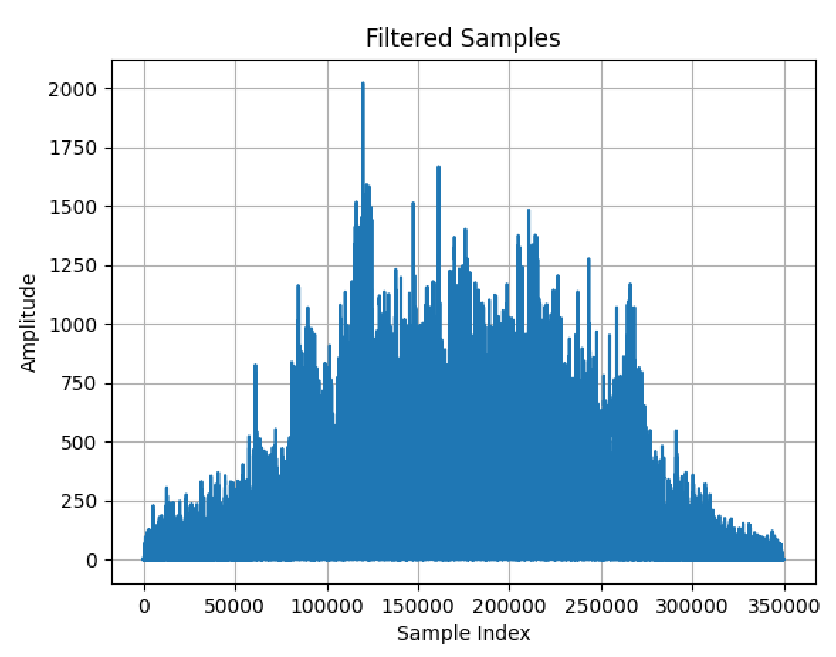
The result of applying a matched filter using both audio signals
Notice the changes within the two axes? The x-axis almost contains 350,000 indexes! The output of the matched filter has N + M - 1 indexes where N is the length of the input signal and M is the length of the template. We now notice the changes in magnitude, where some indexes have values over 1000, meaning that there is a strong correlation and our signal must be a Scrub Jay. The output is strongest in the middle, which is expected because the Scrub Jay is making the clicking noise that we are looking for!
However, our implementation of the matched filter isn't perfect as of late. The noise coming from the other bird in Figure 1 has affected the shape of the output, which is seen by the largest spike having a value of over 2,000. Thus there is a chance for false positives. We must ask ourselves how many false positives are we willing to have because with each false positive we use up the battery in our tag and record void data. To combat this, we could apply thresholding where we see if segments of the output go over a certain value, such as 1000. Perhaps another form of data can be used besides PCM samples. Nonetheless, even with the refinement we must do, we are one step closer to recognizing our beloved Scrub Jay from a tag!