Synthesizing and Verifying a Better FFT
Edmund Lam and Barry Lyu
May 1, 2024
Hi, we're Edmund and Barry, members of the C2S2 digital subteam. Last semester we talked about a complete redesign of the FFT, this post will be a follow-up to our previous blog post, and we will talk about some further optimizations to the FFT, along with a unified testing framework for all different implementations of the FFT module.
The Fast Fourier Transform is an algorithm that converts time-domain signals into their frequency-domain representations. It has many different applications including audio processing, machine learning, etc.
FFT Optimization And Synthesis
Last semester, we made the switch from a Cooley-Tukey FFT to the Pease FFT implementation, it brought a massive increase in performance while using less area. We have made many optimizations from that original implementation and the following is our latest block diagram.
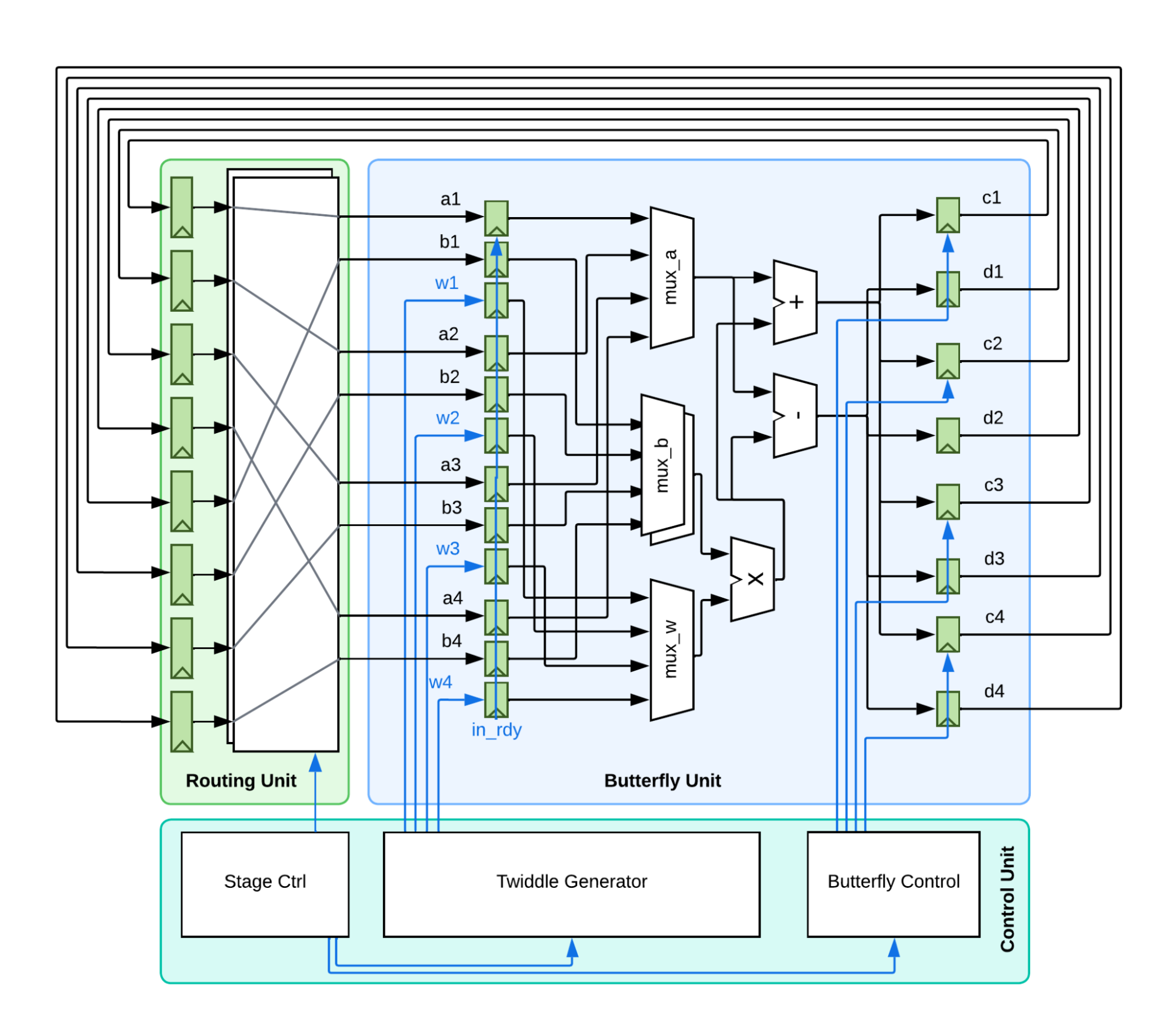
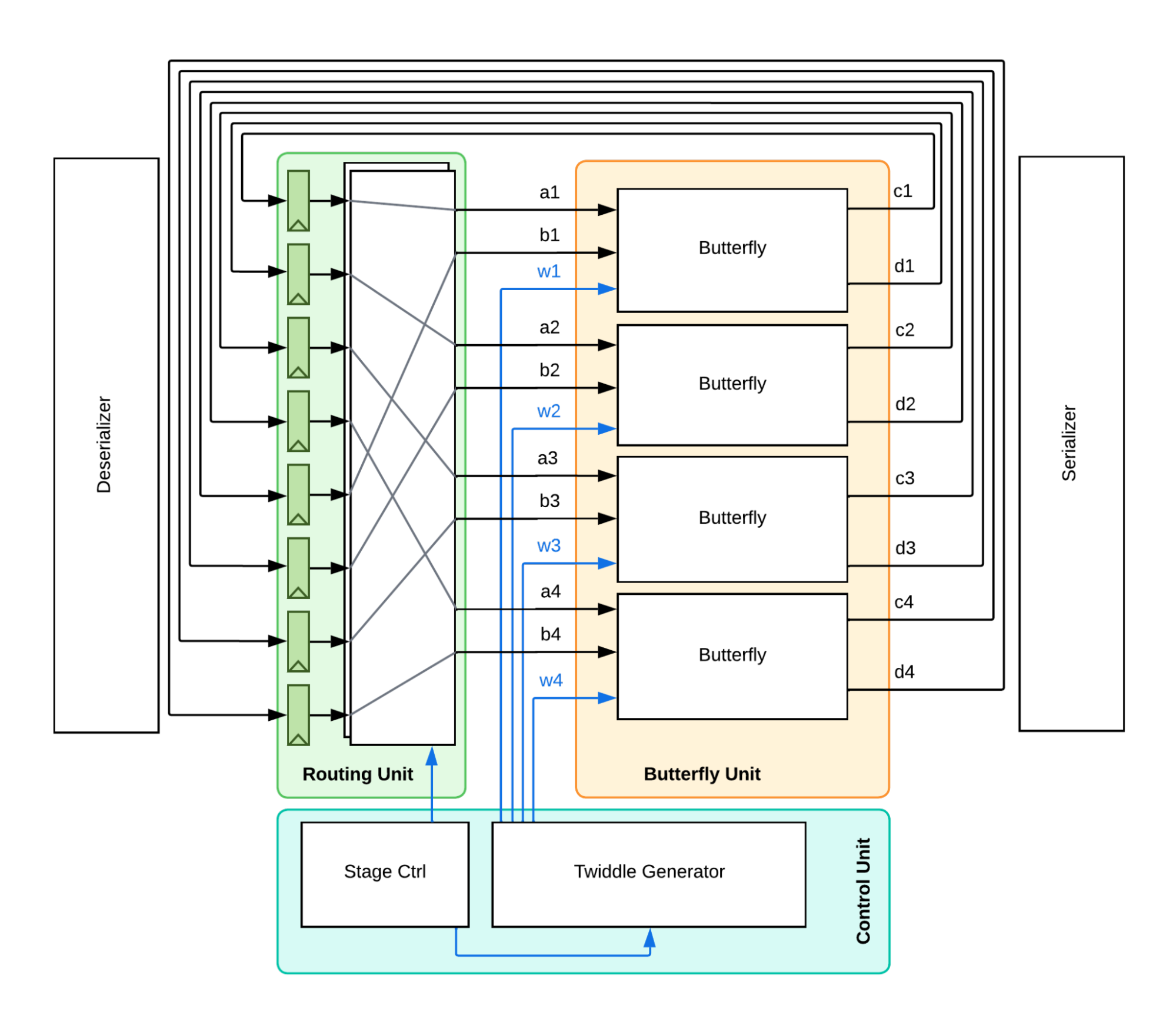
The diagram on the left is our implementation from last semester, and the one on the right is our latest design.
As you might have noticed, we have abandoned the multiplexed butterfly unit because it adds too much routing overhead and stresses our synthesis tools. We now have a butterfly for every pair of inputs, but by doing so, we can also save two sets of registers now that the butterfly is single-cycle.
As you might have noticed, we have abandoned the multiplexed butterfly unit because it adds too much routing overhead and stresses our synthesis tools. We now have a butterfly for every pair of inputs, but by doing so, we can also save two sets of registers now that the butterfly is single-cycle.
We have pushed various different parameterized versions of the FFT through synthesis and the following table shows all the synthesis results.
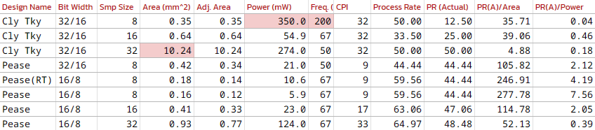
Out of all the different versions, we picked the 32-point Pease FFT with a bit width of 16, because the accuracy of FFT results benefit more from increased kernel width than bit width. Our new FFT operates on a 32-point FFT with almost the same CPI as the 8-point FFT in our tape-in from last year, this would bring accurate frequency results, and help make bird rattle classification more accurate.
Our key takeaway from the FFT is that we should always keep synthesis in mind in writing RTL code, think about the capabilities of the tools, and push through flows early. This helps us understand how different components affect area and methodology, otherwise, we wouldn't know what to optimize for.
Unified FFT Testing Framework
One of our focuses when writing hardware is also thorough testing, not just of the FFT but also of modules and components interacting with the FFT. In our case, we want our FFT to run on audio samples of bird calls, so that a later classification module can decide whether or not to record the audio sample.
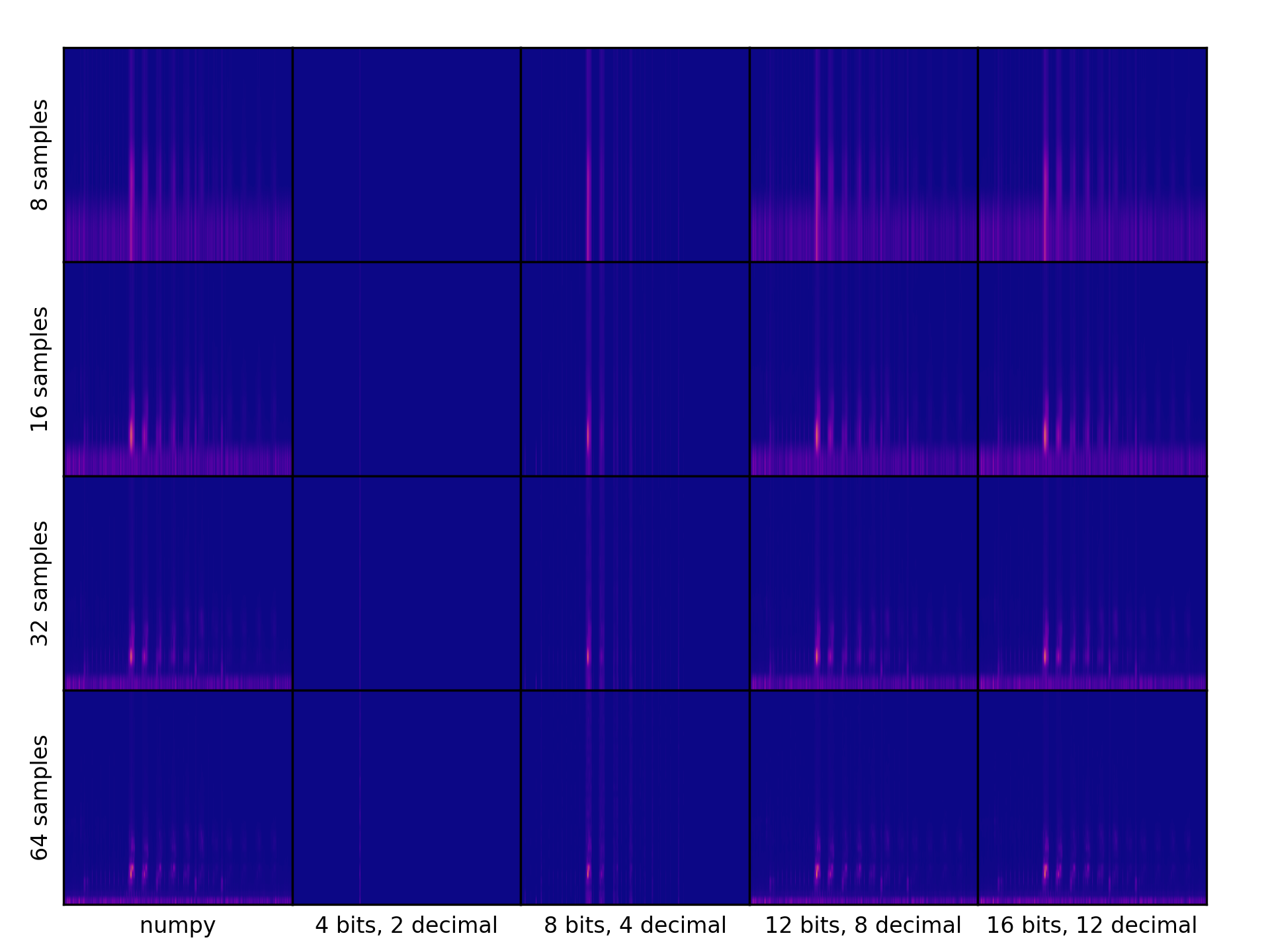
Our old FFT was tested on a combination of manually calculated expected inputs and outputs (mostly for nice single frequency inputs), and a number of randomized tests comparing our outputs against numpy's FFT. While this can be an effective method to test for accuracy, the specifics of our FFT implementation meant our accuracy would vary, not only because of fixed-point arithmetic imprecision but also the order in which math operations were applied. As shown in the diagram below, different amounts of decimal points and different FFT widths can lead to drastically different outputs even given the same input.
The existing method to achieve bit-accurate results is to simulate the FFT in verilator, a very compute-heavy process that is infeasible especially if we want to run the FFT millions of times on actual audio samples. Because of this, testing adjacent components can become incredibly slow and tedious if we have to hook up these modules to the FFT at the RTL level. Because of this, one of the most important parts of designing hardware is in fact designing software simulations- algorithms that perform exactly the same operation as a hardware module. Implementing the same algorithm in both hardware and software can help catch bugs- even if two algorithms are supposed to do the same thing, the thought process in designing for hardware is very different from software, so re-implementing can often lead to mismatches in behavior. This encourages re-evaluation of both algorithms, and can help ensure their accuracy
This is not to say that comparing the two is enough, however- testing against a verified algorithm (such as numpy) and including edge cases are both still important parts of verifying a design. This method of building identical software and hardware modules is helpful especially when it comes to putting together different modules, where a behavioral model written in software can be made by putting together smaller models, just as we would in verilog. Eventually, the goal is to test this software model against both RTL simulations and on the physical silicon, to ensure that behavior is uniform at all levels of abstraction.
One of our biggest takeaways from working with hardware is the importance of testing thoroughly and often. When working with hardware, it is imperative to make sure that code is correct at all levels, which requires thorough tests that can easily be ported to compare many different possible backends, whether it be RTL, Gate level, or the physical die. Many things can lead to mistakes, whether it be undefined behavior in verilog that behaves differently in simulation, or improper resetting that isn't caught at the RTL level. Building abstract software models allows us as designers to reevaluate our algorithms at a higher level, simplifying away some of the intricacies of HDL programming and helping us catch bugs along the way.