Iterative vs. Unrolled Calculations

When determining how to do many of the same calculations in hardware, there are two main approaches we can take. Iterative designs perform the computation using the same hardware, re-using it for all of the iterations of calculations that we need. In comparison, unrolled designs use multiple instantiations of hardware (one for each of the calculations) to "unroll" the calculation across space.

These two approaches lend themselves towards different applications. Compared to unrolled designs, iterative designs use less hardware, as the same piece of hardware is re-used for all calculations. This may make them more appropriate for scenarios where area is at a premium, such as embedded systems. This will also cause them to use less power, as less hardware needs power to run.

However, since an unrolled design has many stages that a given transaction goes through, it can handle multiple transactions at once (with each transaction in a different stage in the design). This is known as pipelining, and allows our unrolled design to handle more transactions overall, having a higher throughput. A good analogy for pipelining is a lunch line. Before each customer has received a complete meal, they must pass through multiple stations to pick up various food items. For example, they might receive a sandwich in the first station, a salad in the second, and a drink in the third. In this lunch line, there is nothing stopping one customer from picking up a salad at the same time the next customer is picking up a sandwich. If our lunch line was iterative, each customer would have to wait for the customer in front of them to pick up all three items before they could pick up their first, which is a funny idea.

These concepts may be hard to grasp at first, so let's do an example! One common operation we might need to do in hardware is multiplication. Let's consider the algorithm below (in pseudocode) for multiplying two 32-bit numbers using many additions:

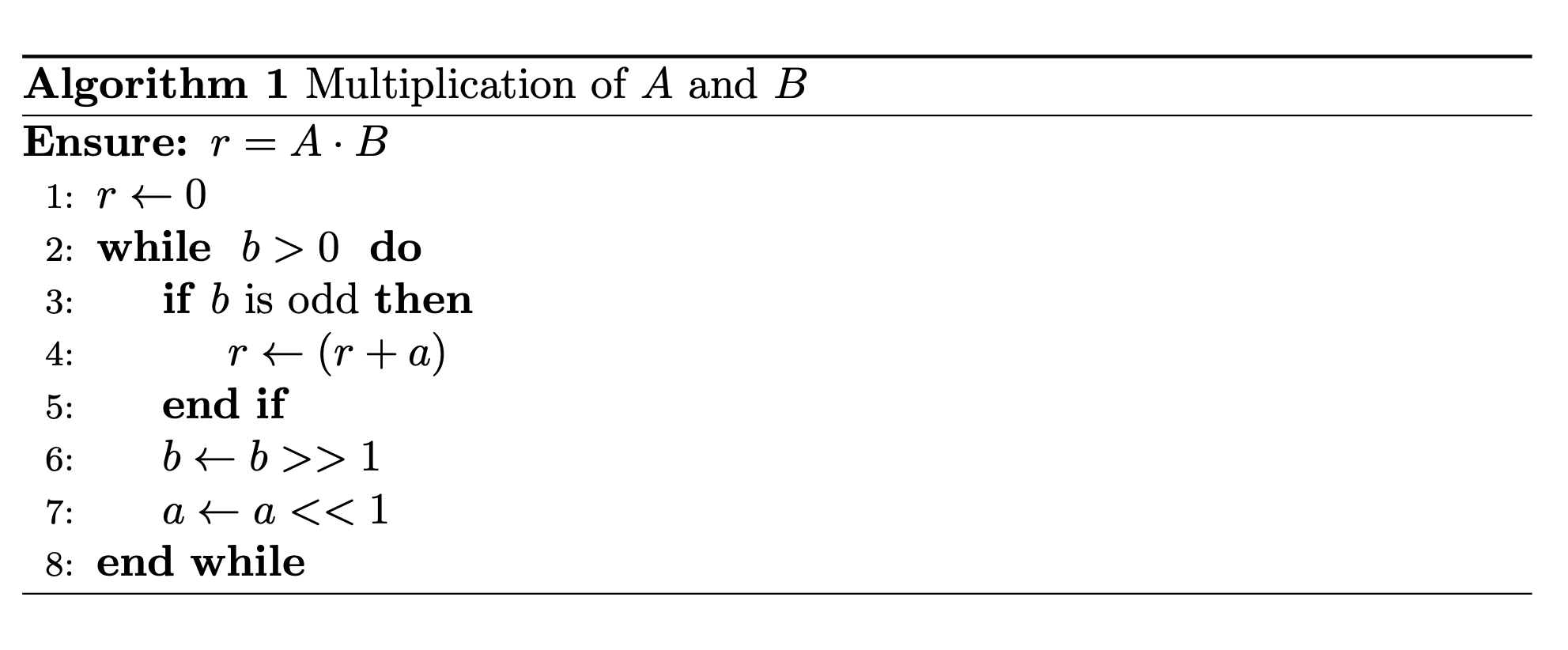
In this algorithm, we start with our result (r) as 0. Then, each operation of the loop, we conditionally increment r by a, depending on whether b is odd (in a binary representation, this is determined by whether the last bit of b is one or not). Finally, we shift b to the right (dividing it by 2), and shift a to the left (multiplying it by two). This is how multiplication is done in binary! For our specific application, since our values are 32 bits, we will need to perform 32 multiplication steps in order to compute the product (optimizations could be made to this to achieve fewer steps, which we won't cover here)

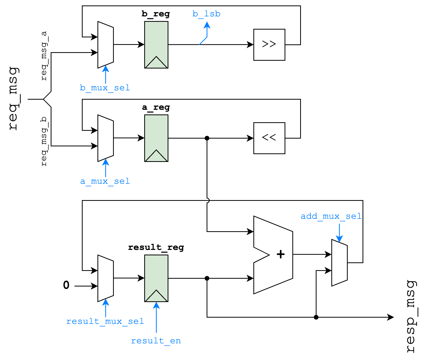
We can see that we need to do the operation inside the while loop many times (we'll refer to one execution of this loop as a multiplication step); we can either do this iteratively, or unroll the operations in hardware. Our iterative datapath is below, adapted from Cornell's ECE 4750. The green elements are registers (used to store values), and the trapezoids are multiplexers (commonly known as muxes), used to select between two values (we won't cover the control logic used to control how data moves, colored in blue, only the elements involved in the actual computation). From here, you can work through the diagram to identify how it corresponds with the above algorithm; notice how it uses the same hardware to perform all of the additions and shifting for each step:

As an alternative, this design could be unrolled in hardware. For this, we can define a module named MulUnit, to execute one multiplication step (one iteration of the while loop). To unroll the operation, we can instantiate one of these for each iteration we need (in our case, 32)

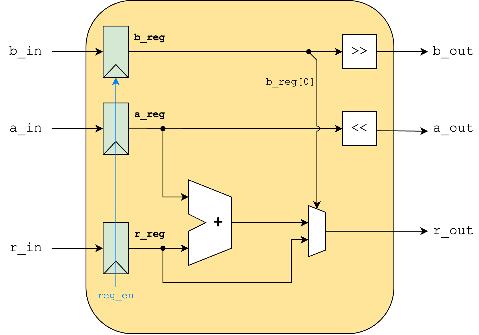
Note how if one transaction is in a particular MulUnit, a separate transaction can be in the MulUnit behind it, with the transactions moving next to each other through each MulUnit in the chain. This demonstrates the pipelining present in the design, and how our unrolled design can handle multiple transactions at once.

To get some concrete results, we can turn our designs into actual metal designs through the use of OpenLANE; this is known as hardening a design, and can inform us about what our design would look like in real life. Below are the two die plots for our two designs; iterative and unrolled:

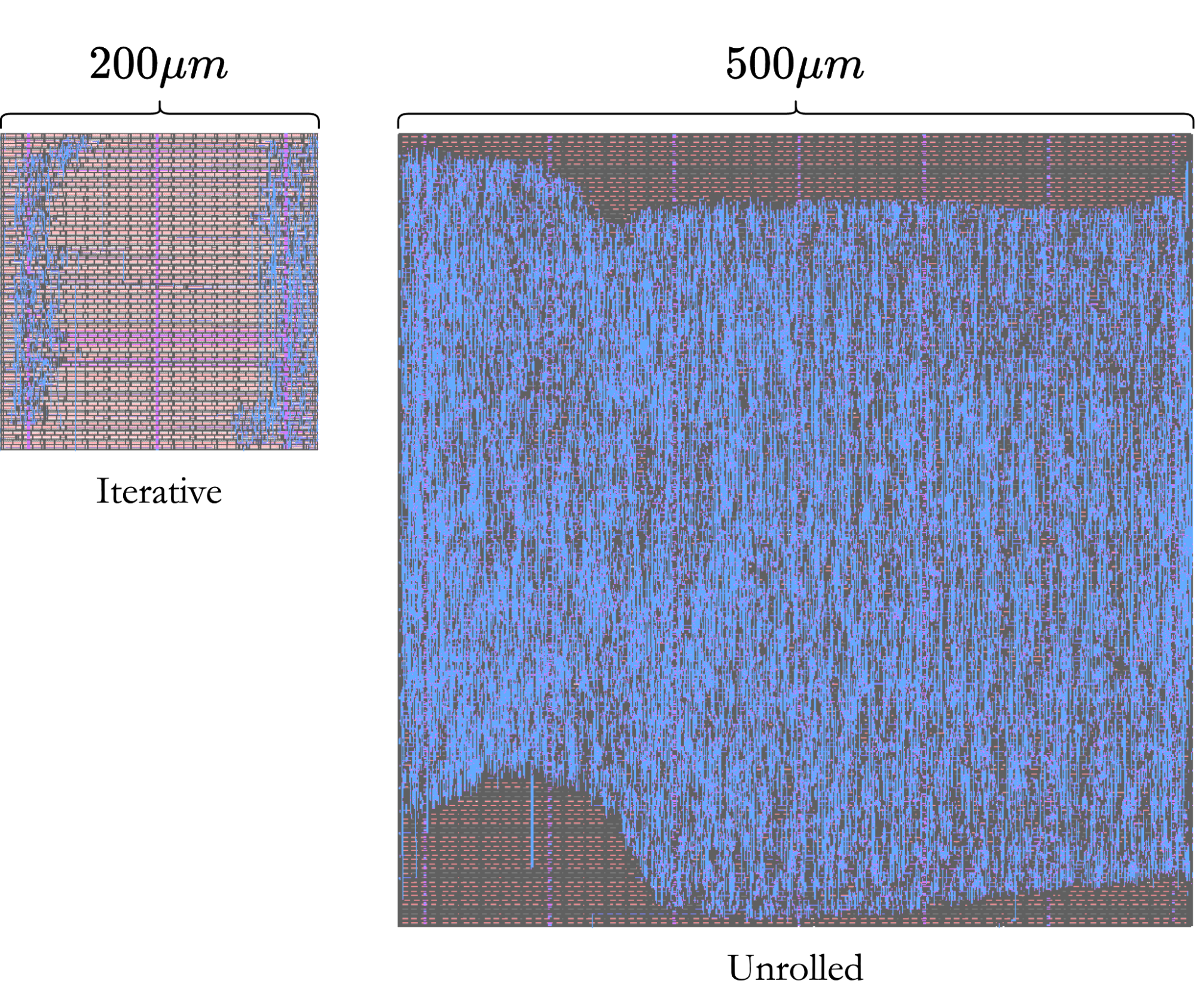
The blue areas (representing wires connecting our design) can give us a rough approximation of where our design is (although some may be hard to see; only dense packets of wires appear at this scale). As expected, our unrolled design uses a lot more hardware. However, our intuition (about 32 times more) is a little off from our results. To make a design, our software often uses cells, which represent individual building blocks (such as an adder, register, etc.). Our iterative design used 430 cells in total, whereas our unrolled design used 9,396 cells, a 21.85x increase. This is likely due to the extra control logic in the iterative design, to make sure that values are directed correctly and that we operate for the correct number of iterations.

Beyond this, we also observe a further discrepancy in the total area used; our iterative design occupies 18,850 mm² with all of its cells, but our unrolled design only uses 58,864 mm² with all of its cells, a 3.12x increase. This is because our unrolled design is not only in a regular pattern (allowing the tools to better optimize the layout), but because there are only local signals; each wire only travels a short distance to the next MulUnit. Conversely, our iterative design features many global signals (signals that travel across the entire design), such as our control logic, which makes it harder for our design to optimize the layout. While the extra hardware and area for our unrolled design may not be quite as bad as we initially thought, it is still a noticeable amount more; we should only use our unrolled design if we can take advantage of the extra throughput, when we're able to have multiple multiplications going at once.

Use in C2S2

Finally, we can take a peek into an instance where C2S2 has faced this tradeoff! As a part of C2S2's collaboration with the Cornell Lab of Ornithology, the digital sub-team has been working on creating a distance calculator. The purpose of this module will be to calculate the distance between a bird and its corresponding base station. As we know, the distance equation derived from the Pythagorean Theorem requires a square root operation. We created a block to calculate the square root of a fixed point value, named fxpsqrt.

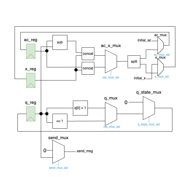
To do this we started by creating a square root calculator for non-fixed-point binary integers. After that, it was time to add fixed-point-support. Our iterative implementation is great because we just need to run the algorithm for more cycles to add fixed point functionality.

The algorithm works by splitting the input bits into pairs of two. For the most significant pair, subtract 01. If the answer is NOT negative, we append 1 to our answer. If the answer is negative, discard the result and append zero to the answer. For the next iteration, we append the next pair of bits to our result and subtract 01 01. We keep doing this until the entire input has been processed.

If we want to calculate the square root of a 32-bit binary integer, the number of cycles required would be the bit width divided by 2 (16 cycles). Now let's say we want to calculate the square root of a 32-bit fixed-point number with 16 fractional bits. We do this by simply increasing the number of cycles by half the number of fractional bits (16 + 8 = 24). This means that inputs of varying size can be handled without making hardware changes. If we had unrolled our iterative implementation, similar to the multiplier example above, the area of our design would have to increase everytime we increased the size of inputs. Although an unrolled architecture would provide higher throughput, it also requires more power and area. Our chip must be low-power and low-area, so an iterative architecture is the correct choice for the square root block, even at the cost of lower throughput (though no impact on the overall transaction delay - the time from start to finish for a given square root calculation)

We also know that the distance formula derived from the Pythagorean Theorem requires multiplication. To do this, we will use the fixed-point multiplier described above. We will continue to refine and optimize this implementation, and look forward to keeping you all updated about the applications of our work!